Laboratory 5: Gesture RC Car

Laboratory Description

I²C sensors are used to further enhance the control developed in Lab 4. A remotely wired compass module is used to directly control the car with hand movements instead of through rotation of potentiometers, among other features.

Laboratory Goals

This laboratory is designed to further a student’s understanding of:

• Using digital sensors to provide feedback,

• Implementing and tuning PID control routines,

Preparation

Students should complete Lab 4 and Activity 14 prior to starting the laboratory.

Hardware and Tools

• RPI-RSLK Robotic Car

• One CMPS12 Electronic Compass

• One SRF08 Ultrasonic Ranger

Description

The speed and turning control inputs as implemented in Lab 4 provided for a direct calculation of the desired straight line and differential turn speeds using potetiometers. This lab introduces digital sensor(s) to provide similar control inputs; however, the sensor(s) are used to determine the cars response to external variable stimuli, as opposed to direct user manipulation. In this case however, the stimuli are still provided through user manipulation.

Instead of having the CMPS12 module mounted on the RSLK, it is mounted on a hand-held breadboard; akin to the mounting of the potentiometers for Lab 4. Movement of the breadboard completely controls the movement of the car: tilting the breadboard forwards and backwards (known as “pitch”) will cause the car to speed up and slow down, respectively. Rotating the about the vertical axis (known as “yaw”) will cause the car to turn left and right, respectively; attempting to turn by the same amount the breadboard does. Additionally, moving the protoboard quickly up or down will enable or disable the motors, respectively; effectively serving as a on/off switch for the control

While the pitch speed control (tipping the sensor forward/back) corresponds nicely with the previously implemented potentiometer speed control of Lab 4; the compass-based turning control requires the car to achieve a specific relative heading. To accomplish this, a Proportional control scheme will be implemented. Note that the wheel speed Integral control routine from Lab 4 should be left unmodified. Alternatively, the wheel speed I control may be disabled for less complexity.

Part A develops portions of the algorithms necessary to implement Part B. One specific algorithm is the method by which the relative heading of the RSLK via the encoders:

Calculation of Car Angle From Encoders

Note

The below discussion describes a proportional+derivative control scheme for controlling RSLK heading. For this semester, the derivate portion my be omitted. This may cause some oscillation in the output control; small amounts of oscillation are acceptable, large oscillations should be fixed.

In this lab, we use the encoders to calculate the relative rotation of the car from an initial starting point (\(0^\circ\)), hence we refer to this measurement as a relative measured heading since an assumed starting point of \(0^\circ\) does not necessarily correspond to a compass direction and only depends on how the car was oriented when initialized.

To calculate the change in angle, we revisit calculations from Measuring Turn Angle from Lab 3; however, we improve these calculations by considering the case where the car can also be driving forward or backwards and not spinning in place. Further, we also assume that when viewing the RSLK movements in small segments, any driven curve can be represented as a circular arc:

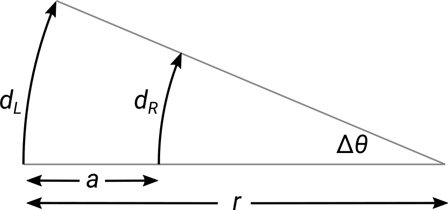
Turn angle geometry

In this figure: both the left wheel and right wheel are shown to travel some distance forward, \(d_L\) and \(d_R\) respectively, the wheels are separated by a length, \(a\) (the RSLK width). Due to the difference between \(d_L\) and \(d_R\) the left wheel traces a circle of radius \(r\), the right wheel traces a circle of radius \(r-a\), and the RSLK turns with an angle change of \(\Delta\theta\). From this diagram, we can assemble the two equations:

\[d_L = r\Delta\theta\]

\[d_R = \left(r-a\right)\Delta\theta\]

Solving for \(r\) in the first equation, substituting into the second equation and solving for \(\Delta\theta\) gives the expression:

\[\Delta\theta = \frac{d_L-d_R}{a}\]

Of course, we can calculate both \(d_L\) and \(d_R\) from how many encoder events have occurred within the considered drive segment and the conversion is the same for each wheel. Therefore, we can modify this equation to instead be:

\[\Delta\theta = \frac{C}{a}\left(n_L-n_R\right)\]

where \(n_L\) and \(n_R\) are the tracked number of encoder events for the considered segment and \(C\) is the conversion factor to convert between encoder events and travel distance: \(d_L = C n_L\) (note: this equation, and specifically the value for C was used/calculated in Activity 11 and Lab 3 and \(a\) is the distance between the wheels). This equation results in \(\Delta\theta\) being in units radians.

Again, this calculation is only applicable for when the change in angle is recalculated often such that only small segments of the drive path are considered (or if the car is driving in a perfect circle). Therefore, to get the actual car orientation angle at time sample \(k\), \(h_{rm}(k)\), the \(\Delta \theta\) values for each drive segment from the start to sample \(k\) must be added together:

\[h_{rm}(k) = \sum_{n=0}^k \Delta \theta (n)\]

This is very similar to how the error sum for I control has been tracked! That is: for each instance where \(\Delta \theta\) is calculated, the calculated value is also added to \(h_{rm}\).

Again, note that this value for \(h_{rm}\) is not the true orientation of the RSLK but a relative orientation considering its initial orientation (that is, the orientation when it was turned on) as \(0^\circ\).

Further, it is possible for this math to produce an angle that is larger than \(360^\circ\); whereas the output of the CMPS12 is always in the range of \(0^\circ\) to \(360^\circ\) (though measured in tenths of degrees: 0-3600). Therefore, it makes sense to ensure that \(h_{rm}\) always fits within this range as well. To this end, the following pseudocode is proposed:

...
new rel. heading = old rel. heading plus calculated delta theta (converted to degrees)
if new rel. heading < 0: add 360 to rel. heading
if new rel. heading > 360: subtract 360 from rel. heading

Finally, it should be understood that although the figure drawn shows that both wheels are traveling in the same direction it is not required for this math to be correct: one wheel may be traveling forward and the other in reverse and the calculations will still hold. This implies that the direction of the encoder events (forward/backward) must be tracked in addition to the total number! As such, encoder events that occur when the wheel is traveling in reverse should be considered “negative” events, which subtract from the total number of events.

The direction of wheel rotation may be determined in one of two ways:

1. If the wheel is being controlled by the program, the specified wheel direction via GPIO may be used, or

2. The second encoders on each wheel, Left/Right Encoder B, may be checked each time an encoder event occurs to determine direction (as discussed in Timer Capture/Encoders lecture). The current iteration of RSLK cars in the classroom; however, do not have this encoder connected by default and therefore this method may not be feasible.

Angle-Based Turn Control

The angle-based turn control for Part B of this lab assumes the same method to turn control used previously, where the desired speed is manipulated with a differential speed between them that causes a rotation:

\[v_l = v_d - \Delta v~~~~v_r = v_d + \Delta v\]

where \(v_d\) is the desired speed, \(v_l\) is the desired left wheel speed, \(v_r\) is the desired right wheel speed, and \(\Delta v\) is the steering control speed difference used to turn the car. As opposed to potentiometer however, the value for \(\Delta v\) is now calculated from the difference between a desired heading and the relative measured heading using a proportional and derivative control scheme:

Steering control system

Continuous control equation:

\[\Delta v(t) = k_P^h \epsilon_h(t) + k_D^h \frac{\mathrm{d}\epsilon_h(t)}{\mathrm{d}t}\]

Discretized control equation:

\[\Delta v(k) = k_P^h \epsilon_h(k) + k_D^h \left(\epsilon_h(k) - \epsilon_h(k-1)\right)\]

where \(k_P^h\) is the steering proportional gain constant, \(k_D^h\) is the steering derivative gain constant, and \(\epsilon_h\) is the heading error.

Calculation of the heading error is not simply the difference between the desired heading, \(h_d\) (measured from hand-held CMPS12), and the relative measured heading, \(h_{rm}\) (calculated via encoders measurements):

\[\epsilon_h = \left( h_d - h_{rm} \right) ~~~ \leftarrow \mathrm{wrong~by~itself}\]

as heading is a periodic function and is not necessarily linear; namely, the value for heading goes from \(0^\circ\) to \(359^\circ\) and then back to \(0^\circ\). This may result in erroneously large values for \(\epsilon_h\). For example, if \(h_d = 330^\circ\) and \(h_m = 60^\circ\) the direct calculation leads to \(\epsilon_h = 270^\circ\), which would cause the car to turn in the wrong direction towards the desired heading; that is, the long way. Of course, any angle in degrees is equivalent to itself \(\pm 360^\circ\), which may be used to correct the calculated \(\epsilon_h\) to determine the shortest direction to turn to reach the desired heading (three lefts make a right!). Applying to the previous example, the correct error would be \(\epsilon_h = 270^\circ - 360^\circ = -90^\circ\). It is necessary to always minimize the absolute value of \(\epsilon_h\). Since the value of the error may only be changed through \(\pm 360^\circ\), then the absolute value of the error must be bounded by half of that value: \(\left|\epsilon_h\right| \leq 180^\circ\), leading to the pseudocode:

heading error = desired_heading - measured_heading
If heading_error > 180 degrees
    Subtract 360 degrees from the heading_error
If heading_error < -180 degrees
    Add 360 degrees to the heading_error
...
continue control scheme

This is known as “wrapping” the angle to the \([-180^\circ,180^\circ]\) domain. Note that this should only be done with the calculated error, not the individual values for \(h_d\) and \(h_{rm}\)!

Similarly, the derivative of the error will suffer from the same when the error wraps around the \(\pm 180^\circ\) boundary in subsequent samples. However, this case only occurs when the car has a significant error, which is not generally expected when the program is operating correctly. Therefore, correction of the derivative error is neglected.

Part A

For this part, the lab’s required circuit is built and speed control is implemented. On/Off control is also added.

Circuit:

Using the same long wires used in Lab 4 and the I²C circuit from Lab 5, build the required hardware: the CMPS12 is to be mounted on the remote breadboard and connected to the I²C bus, with pull-up resistors mounted on the RSLK or hand-held breadboard. Please do not take the CMPS12 with you when leaving the classroom as there are not enough for each group to keep one at all times.

Warning

Repeated: Please do not take the CMPS12 out of the classroom: either leave them on the car or return them to their box/tray in front of the podium.

Program:

Copy and modify your completed Lab 4 to remove the ADC and potentiometer dependencies; replacing the straight-line desired speed with measurements of the CMPS12 pitch register (see Electronic Compass, ADDR: 0x60 and CMPS12 Datasheet), where the CMPS12 is read using the same I²C module and functionality from the previous activity. Specifically, the program should read the pitch register measurements and convert it into desired speed, \(v_d\). Your math from Lab 4 will need to be adjusted to account for the different values returned by the CMPS12. At this point in the lab, the differential speed, \(\Delta v\), should be set to 0 such that no turning occurs.

Note

The pitch measurement speed control should behave with the same type of response as from Lab 4, specifically: The speed control should have the car stop if the desired speed is less than \(10\%\) duty cycle and should be limited to a maximum duty cycle of \(50\%\).

It is up to the groups to determine a reasonable conversion between pitch angle and desired speed.

In addition to the above, the CMPS12 measurements should also be used to control the driving state of the car:

On/Off Control

The RSLK will have two states in this lab:

1. Enabled (On): Car operates as expected, with motors controlled by CMPS12 pitch and heading, and

2. Disabled (Off): Car remains stationary regardless of CMPS12 pitch and heading.

Where transitioning between these two states is done by rapidly raising up the remote protoboard (transition to Enabled state) or moving down the protoboard (transition to Disabled state) over a 3-6 inch range. These movements may be detected via the accelerometer outputs of the CMPS12; specifically, the axis aligned to the up/down direction can measure the movement of the protoboard on that axis. The direction of movement/acceleration will be identified by the sign of the output.

Upon startup, the car should enter the default Disabled state with the RGB LED lit red. When a large upwards acceleration is detected, the program should light the RGB LED green and then delay for 1 second; ignoring all outputs of the CMPS12 (namely to ignore the accompanying deceleration of the movement) before transitioning to the Enabled state. Similarly, detection of a large downwards acceleration should trigger a change to the Disabled state with a 1 s delay and RGB LED set back to red.

The correct axis to monitor for this acceleration signal, and a corresponding suitable trigger value, should be determined by the group by measuring all CMPS12 acceleration values and printing them to the serial console. The CMPS12 can then be moved in the desired way with these values monitored.

Checkoff

Demonstrate that the CMPS12 pitch can properly influence RSLK drive speed and the On/Off control works well. Printing of suggested values above may be requested.

Warning

Failure to return the CMPS12 to the RSLK or podium when leaving the classroom may result in the revocation of Part A credit.

Part B

This part of the lab should be assembled in a specific order in order to verify pieces before assembly of the whole program.

Calculate Relative Measured Heading

Generate the relative measured heading, \(h_{rm}\), as defined in Calculation of Car Angle From Encoders. To do so, you must:

1. Modify the tracking of the total encoder events such that if the wheel is traveling in the forward direction, events are added to the total. If the wheel is traveling in the reverse direction, events are subtracted from the total. This may be done simply by tracking the enforced direction of the motors.

   Hint

   Because of the subtraction in reverse for tracking events, the variables storing the total number of encoder events must be signed: int32_t instead of uint32_t.

2. Calculate the values for \(\Delta \theta\) and \(h_{rm}\) each time the control loop runs.

3. After the calculation for \(\Delta \theta\): reset the encoder events counters such that they are only tracking the number of events between control loop iterations. This would determine the “drive path segment” considered, as discussed above. If a running total of encoder events is still desired, another variable may be used instead for the segment tracking.

The calculation above may be tested with the motors off: set the car on the bench and move it manually by hand forward with turns while also printing out the calculated value of \(\theta\) after each control loop iteration. If the calculations are correct, the car should report fairly accurate orientation changes. Please be gentle when moving the car by hand: abrupt and strong movements wear the gear train clutch within the motor housing.

Note that the calculation of \(h_{rm}\) done here will be in radians unless modified!

Note

Note that the instructions above say “forwards with turns.” This is because wheel direction is not directly measured here and as such, we want to ensure that both wheels travel in the same direction for this measurement.

Add Angle-Based Turn Control

Implement the angle-based turn control as described in Angle-Based Turn Control. If \(h_{rm}\) is calculated in radians, it must be converted to match the units of the CMPS12 heading measurement: tenths of degrees (0-3600).

This control should follow the pseudocode:

Calculate the heading error and "wrap" the error to -180 to 180 (or -1800 to 1800)
Calculate the differential speed using the P control (equation given above)
Enforce maximumum limit on differential speed to 20 % duty cycle

Note

No derivative control is required here. For this semester, we are not requiring implementation of derivative control.

To tune the proportional control gain, start with a very low value and incrementally increase it until the car behaves nicely.

All other control specifications are carried over from Lab 4:

Control Specifications (generally same as Lab 4)

Quantity	Value	Notes
Max |Diff Speed|, \(\Delta v_{max}\)	20 %	Set | \(\Delta v\) | to this if greater than
Min |Speed|, \(v_{d,min}\)	10 %	Set |desired speed| to 0 if less than
Max |Speed|, \(v_{d,max}\)	50 %	Set |desired speed| to this if greater than
Min PWM DC %	10 %	Set compare value to this if less than
Max PWM DC %	90 %	Set compare value to this if greater than
Control Routine Period	50 ms

Checkoff

With all components listed above completed, demonstrate the full functionality as described. Minor car oscillation around the desired heading is acceptable. Printing of suggested values above may be requested.

When complete, submit the code to Gradescope.