Laboratory 4: “Remote” Control Car¶

Laboratory Description¶

In this lab, the car is programmed to drive in response to control inputs via a “remote” control with two potentiometers, one each controlling speed and direction.

Laboratory Goals¶

This laboratory is designed to further a student’s understanding of:

Using an analog to digital converter to measure inputs,

Implementing and tuning an I control routine.

Preparation¶

Students should complete Activities 11 and 12 prior to starting the laboratory.

Hardware and Tools¶

TI-RSLK Robotic Car
2x 10 kΩ potentiometers
[optional] 1x photoresistor (photocell) and 1x 2-3 kΩ resistor

Project Template¶

lab4_template.zip * Read comments thoroughly!!!
Or use Lab 3 code with speed control removed (encoder calculations left intact).

Description¶

This lab entails programming the car to act like a “remote controlled” car, though the remote in this case will simply be a wired protoboard. Below is a figure describing this configuration (in the style of xkcd).

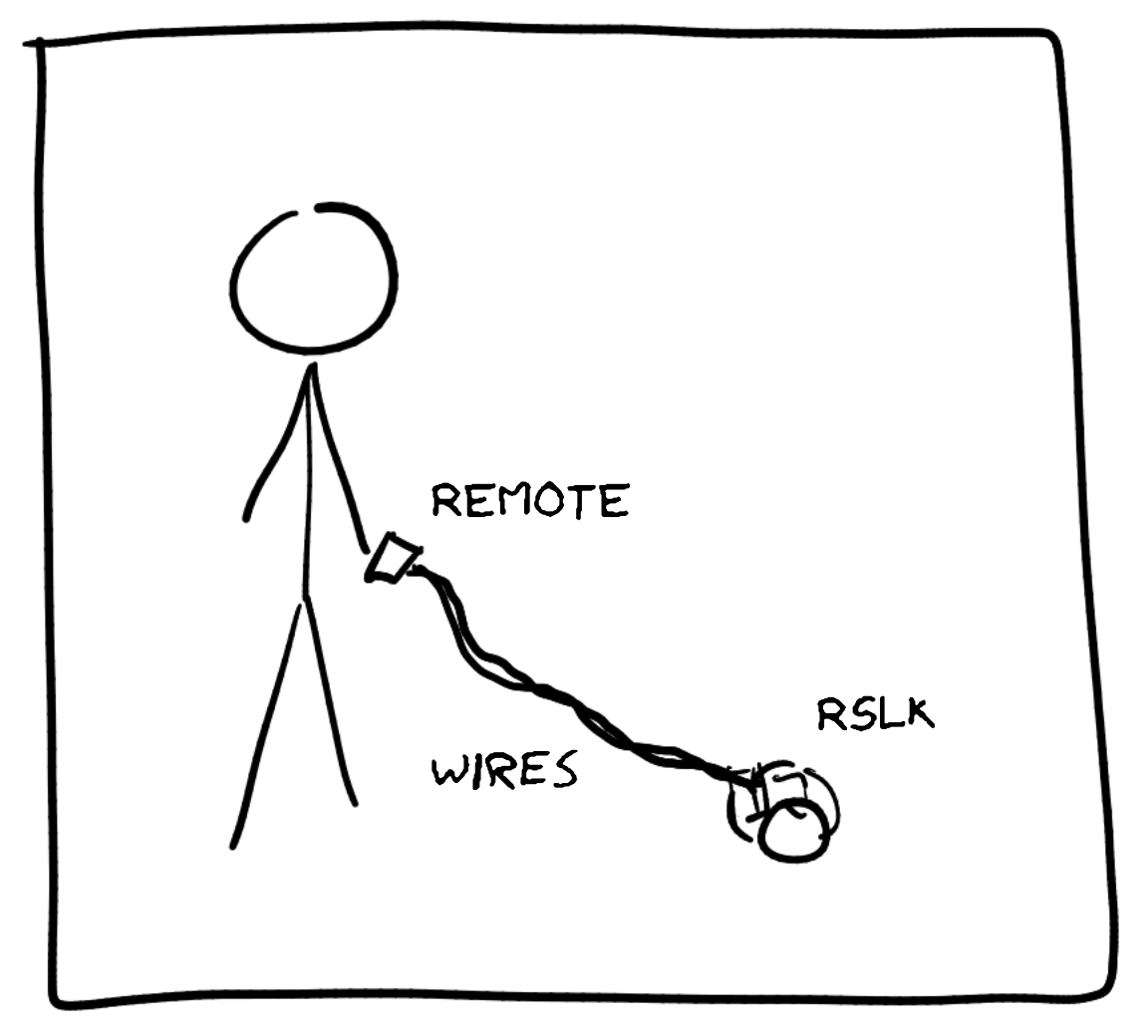
The remote, which is directly wired to the RSLK using long (e.g., 1 m long) wires, is built such that there are two potentiometers, one which controls the speed of the car and the other controls the turning direction. The potentiometers provided in the lab are easy to turn with fingers only and rotate only over 180°, making them a decent part to use as a control knob. Do not use the potentiometers from the ADALP2000 parts kit for this! Both of the potentiometers should be set such that the midpoint of their rotation is facing away from the user. The functionality of the potentiometers is described in the figure below.

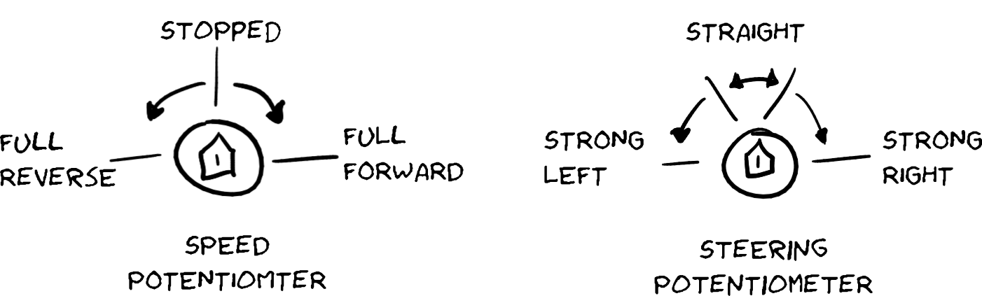
As shown, the speed control potentiometer will will cause the car to be stopped when the wiper is at the midpoint and rotating it clockwise will increase the speed of the car in the forward direction. Similarly, rotating it counter clockwise will cause it to increase in speed in the reverse direction (backwards). Centering the turning (steering) potentiometer will cause the car to drive straight. Driving straight is enforced within a range around the steering potentiometer and not just when it is perfectly centered. Outside of this zone, turning clockwise will cause the car to turn right (or left if driving in reverse). Likewise, turning the potentiometer counter clockwise will cause the car to turn left (or right if driving in reverse).

As the speed of each wheel is adjustable, the wheel speed control must be capable of quickly acclimating to new values. The speed control as used in Lab 3 was effective in producing consistent speed between both the left and right wheels; however, the method used would be very slow to adjust with changing desired speeds. This laboratory presents the use of Integral (I) control to realize a more effective control scheme towards driving the car at non-constant rates.

To follow the half-circle ends of the track, the car must also be able to turn in a curvilinear fashion, as opposed to in one spot as in Laboratory 3: Predetermined Paths. One method to produce a smooth turn is to control the wheels in a differential fashion. The full control scheme for the lab is presented in the following sections.

ADC and Potentiometers¶

Potentiometers are variable resistors (simplified) that may be used as variable voltage dividers:

Resistor (left) and potentiometer (right) voltage dividers¶

A potentiometer has a total resistance, \(R_{pot}\) which is split into “legs”; e.g., \(R_1\) and \(R_2\), such that \(R_{POT} = R_1 + R_2\). The legs are split by the potentiometer’s “wiper”, which is basically a sliding contact along the \(R_{POT}\) resistor, commonly shown in schematic symbols as an arrow. As the wiper is moved up and down on \(R_POT\) (the potentiometer being rotated), the values of \(R_1\) and \(R_2\) will change, resulting in a changing output, where \(V_{out}\) is the voltage on the wiper:

\[V_{out} = V_{in} \frac{R_2}{R_1 + R_2} = V_{in} \frac{R_2}{R_{POT}}\]

Given this functionality, potentiometers are used very often as control knobs. For this lab, the 3.3 V source should be used as Vin and Vout is attached to a GPIO pin configured as an analog input.

As this lab requires the use of two potentiometers, the ADC14 must be configured to be capable of reading both inputs. This will require two ADC_MEMx locations to be configured (one for each potentiometer). With two memory locations configured. It is suggested to use Multi Sequence Mode, as used in Activity 11, to support multiple measurements:

Using multi sample mode in manual trigger mode (repeatMode = false):
- [Do once] Use bool ADC14_configureMultiSequenceMode() to select the ADC_MEMx locations (and associated inputs) to convert,
- Trigger a conversion of both channels with bool ADC14_toggleConversionTrigger(),
- Wait for the conversion to complete by continually checking bool ADC14_isBusy(), and
- Read the result of both conversions by calling uint16_t ADC14_getResult() for each input.
Using multi sample mode in continuous trigger mode (repeatMode = true):
- [Do once] Use bool ADC14_configureMultiSequenceMode() to select the ADC_MEMx locations (and associated inputs) to convert,
- [Do once] Trigger the continuous conversions to start with bool ADC14_toggleConversionTrigger(),
- Read the results when needed by calling uint16_t ADC14_getResult() for each input.

See the ADC14 DriverLib Documentation for an in depth description of each function’s usage.

Wheel Speed Control¶

The wheel speed control specified here replaces the incremental control used in Lab 3 to cause the car to drive straight at a constant speed. This version is a hybrid control system; where:

an open loop portion is used to provide immediate speed modification when a change of speed is requested via the potentiometer. This portion may be viewed as an open loop proportional (unity) gain control, and
an Integral control portion is implemented to compensate for wheel speed errors between the desired speed and the actual speed; useful in reducing the speed difference between the left and right motors.

The control system is described in the figure below.

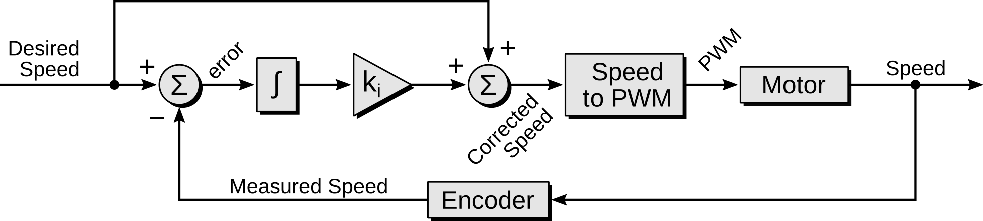
Wheel speed control system¶

Mathematically, the control scheme presented in the above diagram may be written as:

\[v_c = v_d + k_I \int \left(v_d - v_m\right)\, \mathrm{d}t\]

where \(v_d\) is the desired speed, \(v_m\) is the measured speed, \(v_c\) is the corrected speed, and \(k_I\) is the integral gain constant. The two portions of this control system are the two terms in this equation: the open loop speed, \(v_d\), and the integral component, \(k_I \int \left(v_d - v_m\right)\, \mathrm{d}t\). The error, as noted in the block diagram, is simply the difference between the measured and desired speeds: \(\epsilon = v_d - v_m\).

The control equation provided above is in continuous form. It is necessary to use a discrete form in the program:

\[v_c(k) = v_d(k) + k_I \sum_{n=0}^k \left(v_d(n)-v_m(n)\right)\]

This version assumes that the control equation is evaluated on a constant time interval; otherwise, a \(\Delta t(k)\) term must appear in the summation. It is necessary for the control equation to operate on a time scale that is meaningful to the integral control; that is, the car should be able to respond to the previous input before acting on a new error value. This implies that the control equation should be run at approximately the motor response rise time or greater. Values for this range from 50 ms to 300 ms (roughly). For this lab, it is suggested to evaluate the control equation every 100 ms.

This control equation may be used to operate on many measures of the speed; for example: the wheel rotation speed (rpm), the linear speed (m/s), etc. In this instance, we make the assumption that the PWM and its associated duty cycle are valid “measures” of speed; that is, the actual wheel speed will be proportional to the duty cycle. This allows us to formulate the speed in terms of the duty cycle:

Duty Cycle to Speed Mapping¶
Duty Cycle	Speed
-100 %	Full Speed Reverse
0 %	Stopped
100 %	Full Speed Forward

With \(v_d\) and \(v_c\) in duty cycle units, the PWM Compare Value to apply to the wheel may be easily calculated knowing the PWM .timerPeriod.

The above requires that the output of the Encoder be converted into duty cycle units to produce \(v_m\) in order to complete the feedback path. This conversion is provided empirically: the figure below shows a characterization of the encoder response versus a PWM duty cycle along with a rough trendline match of the data (red) 1.

Encoder convertion to speed (duty cycle).¶

The equation for this above trendline is:

\[N_{enc} = \frac{1500000}{DC [\%]} \rightarrow v_m = DC_m [\%] = \frac{1500000}{N_{enc}}\]

where again, the “measured speed,” \(v_m\), is equal to the “measured duty cycle,” \(DC_m\), and \(N_{enc}\) is the encoder counts.

Pseudocode for the implementation of this control system is provided in the Implementation Guidance section.

1: This data was generated by applying a fixed PWM duty cycle to a motor (unloaded) and then measuring the steady state output.

Turn Control¶

The car turn control for this lab assumes that there is a desired speed that the car must maintain while also turning. This implies that the wheels must have different speeds to cause a rotation while also averaging to the desired speed:

\[v_l = v_d - \Delta v~~~~v_r = v_d + \Delta v\]

where \(v_d\) is the desired car speed, \(v_l\) is the desired left wheel speed, \(v_r\) is the desired right wheel speed, and \(\Delta v\) is the differential speed used to turn the car. The definition of speeds above implies that a positive \(\Delta v\) would result in a left turn.

If it is assumed that the wheels do not slip, then the wheels must travel in concentric arcs during the turn:

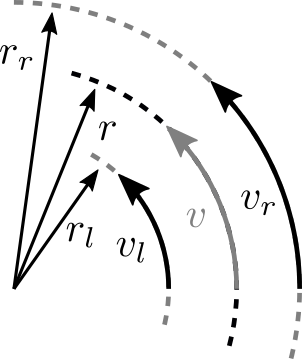
Turn radius due to differential wheel speed¶

This implies that the wheels and car center will be travelling at the same angular turn speed, \(\omega_t\), around some center point. Knowing that an arc length may be calculated as

\[s = \theta r\]

then taking the time derivative of the equation results in the relationship

\[v = \omega r\]

Again, since \(\omega_t\) is shared between the wheels and center of the car, then

\[\frac{v_l}{r_l} = \frac{v}{r} = \frac{v_r}{r_r}\]

Since the distance between the wheels, \(d_w\), is known or can be measured, \(r_l\) and \(r_r\) can be defined as:

\[r_l = r - 0.5 d_w~~~~~~~~r_r = r + 0.5 d_w\]

Using the above equations, \(v_l\) and \(v_r\) can be solved for:

\[v_l = v_d \left( 1 - \frac{0.5 d_w}{r} \right)~~~~~~~~v_r = v_d \left( 1 + \frac{0.5 d_w}{r} \right)\]

This implies that the differential speed, \(\Delta v\) may be calculated as

\[\Delta v = v_d \frac{0.5 d_w}{r}\]

As clear from this equation, \(v_d = 0\) would result in \(\Delta v = 0\), not allowing the car to turn, or the turn radius must be also set to \(0\) (turning without moving forward or backwards). For the purposes of this lab, it is desired to always allow the car to turn. As such, the calculated \(\Delta v\) from the steering potentiometer must be made independent of \(v_d\). To do this, consider the car driving at some maximum speed, \(v_{d,max}\) and a minimum turn radius, \(r_{min}\). Using these, a maximum differential velocity, \(\Delta v_{max}\), may be found:

\[\Delta v_{max} = v_{d,max} \frac{d_w}{2 r_{min}}\]

The value calculated above is then always the used for the maximum value of the differential speed regardless of the set desired speed; where the differential speed calculation uses this value and the steering potentiometer to generate a linearly increasing desired differential speed as the steering potentiometer is turned further off center.

Implementation Guidance¶

While the theoretical implementation of the wheel speed control and the turn control is fairly straight forward to build, several problems arise in the actual implementation, mostly attributed to the functionality of the encoders.

Issue 1: The encoder measurements have a significant amount of variation over a 6 sample cycle. It is strongly advised to average the encoder output over 12 cycles (same as Lab 3).

Issue 2: The encoder measurements are not continuous. This is generally not a significant issue when the car is moving; however, when the car is stopped or moving slowly, the control may use outdated values for the encoder. This will have adverse effects on the integral portion of the speed control. This problem may be reduced by disabling the integral control at very low speeds.

Issue 3: The RSLK will not move with low duty cycles. Therefore, it is useful to force the desired speed to 0 if it desired speed is below a minimum threshold.

Considering the control schemes presented and the issues and solutions provided above, the following pseudocode is the suggested method for implementing this laboratory.

Global variables/prototypes/etc.

main:
    Initializations

    Enforce a startup delay of 1 second (__delay_cycles(24e6))
    Turn on the motors

    Infinite while loop:
        If 100 ms has passed:

            Trigger the ADC to read both potentiometers
            Convert the speed potentiometer measurement to a desired speed
            Ensure the desired speed follows the control specifications below
            Convert the steering potentiometer measurement to a differential speed
                following the specifications below.

            <-- Start Wheel Speed Control -->
            For Each Wheel:
                calculate desired wheel speed as desired speed +/- differential speed
                if |desired wheel speed| is less than minimum value,
                    set the desired wheel speed and compare value to 0
                otherwise:
                    set wheel direction depending on sign (+/-) of desired wheel speed
                    calculate the current speed error from the encoder and |desired wheel speed|
                                 (use trendline equation from figure for current speed)
                    add current speed error to an "error sum" variable (tracking integral error)
                    calculate the corrected speed using the discrete equation above (should be >= 0)
                    convert the corrected speed (duty cycle) into a compare value
                    enforce minimum and maximum limits on the compare value
                apply the compare value
            <-- End Wheel Speed Control -->

 Other Functions:

 GPIO Init (usual stuff)

 Timer Init:
     PWM Timer+CCRs (24 kHz, OUTPUT_RESET_SET <- makes control easier)
     Encoder Timer+CCRs
     100 ms Timer

 ADC Init:
     Fill in as needed

 Encoder ISR:
     Generally the same as in Lab 3 except no incremental PWM control.
     Still perform 12 sample averaging for both encoders but save averages
                          to global variables (for use in control above)

 100 ms Timer ISR:
     Mark that 100 ms has passed using a global flag

Control Specifications¶

Control Specifications¶
Quantity	Value	Notes
Min \|Speed\|, \(v_{d,min}\)	10 %	Set \|desired speed\| to 0 if less than
Max \|Speed\|, \(v_{d,max}\)	50 %	Set \|desired speed\| to this if greater than
Min PWM DC %	10 %	Set compare value to this if less than
Max PWM DC %	90 %	Set compare value to this if greater than
Minimum turn radius, \(r_{min}\), at \(v_{d,max}\)	0.2 m

Part A¶

Wire the potentiometers to P4.1 and P4.4 on your protoboard. Cut long lengths of wire (several feet) to connect the potentiometers to the car. Note that you only need 4 total wires to accomplish this.

Implement the wheel speed control with speed potentiometer input for one wheel only. The other wheel during testing should not be enabled or moving. You will need to generate a conversion equation that maps the ADC output to a desired speed, following the requirements in the control specifications table above. It is suggested to use float type variables for all pieces of the speed calculation to allow more accurate and non-integer values of duty cycle.

Hint

The “conversion equation” noted above for determining the desired speed could be in the form \(y = m x+b\).

A first step in verifying the control operation will be to specify \(k_I = 0\) to test the open loop control portion. This should result in the car spinning the wheel at roughly the right speed but likely have some error. Print out the desired speed, \(v_d\), and encoder measured speed, \(v_m\), (both in PWM Duty Cycle “units” as described) to verify.

Once this is shown to work, \(k_I\) should be set as a non-zero small number, and increased until acceptable operation is achieved:

A too low value of \(k_I\) will resemble the response with \(k_I = 0\).

A too high value of \(k_I\) will result in the wheel misbehaving (e.g., jerking between fast/slow, not settling on correct speed)

A good value for \(k_I\) will result in the wheel setting to the desired speed quickly.

A suggested start value for \(k_I\) is 0.001 (float!), increasing by a factor of 10 for each test and then fine-tuning when the correct magnitude is found.

When testing your control scheme, it is useful to print out many quantities each cycle:

Initial Desired Speed

Modified Desired Speed (after applying minimum/maximum thresholds)

The encoder “measured speed,” \(v_m\), (duty cycle “units”)

speed error summation (integral error)

Corrected Speed, \(v_c\), (duty cycle “units”)

PWM compare value

If, when operating at a constant speed, the speed error summation does not stabilize (e.g., continuously increases or jumps by very large amounts up and down), it is possible that \(k_I\) should be negative for your implementation. Also, make sure that the variables used for each portion of the control make sense and you aren’t getting (1) integer overflow or (2) integer division to 0.

While it is feasible to use your completed lab 3 code as a starting point for lab 4, it is strongly suggested to use the provided template project: lab4_template.zip. If you prefer to use your lab 3 code, ensure that ensure that the previous version of speed control is removed from the Encoder_ISR() while keeping the 12 element averaging, with the final average stored as a global variable.

Checkoff¶

Demonstrate that the speed control potentiometer successfully controls a single wheel of the RSLK (other wheel is OFF) from -50% duty cycle speed to 50% duty cycle speed. The wheel should stop when the potentiometer is centered. A terminal printout of the Desired Speed, \(v_d\), the encoder measured speed, \(v_m\), and corrected speed, \(v_c\) must be provided showing convergence of \(v_d\) and \(v_m\).

Part B¶

Copy the wheel speed control to the other wheel and enable it. Again verify that it works properly by disabing the already verified wheel and testing. Once complete, enable both wheels and ensure the car drives straight with changing desired speeds. Slight turns are acceptable when large speed changes are requested but the car should straighten quickly.

Add turning control to the car once the car can drive straight. The car should not turn if the steering potentiometer is within ±15° of center and then should linearly increase turn strength (differential speed) with increasing potentiometer angle. The maximum turn radius will change with varying desired speeds; however, the maximum turn strength (again, differential speed) should be consistent across all desired speeds. With this configuration, the car should be capable of spinning in place when the speed potentiometer is set to cause the RSLK to stop.

Checkoff¶

Demonstrate the additional components as described above. Submit your final code to the Gradescope assignment.

Do not discard your long wires! They may be used in Lab 5.