Laboratory 3: Predetermined Paths
Laboratory Description
In this lab, the car is programmed to follow a set of pre-planned paths, selected from a bumper press.
Laboratory Goals
This laboratory is designed to further a student’s understanding of:
Implementation of a program with distinct states.
Using timers to produce pulse width modulated signals and measuring encoder outputs.
Performing simple feedback control.
Preparation
Students should complete Activities 10 and 11 prior to starting the laboratory.
Hardware and Tools
RPI-RSLK Robotic Car
Description
Automated systems commonly have to follow a set of predetermined steps in order to meet a goal. The goal in this lab is to cause the car to reach a target location and stop while following a specific route. There are two routes the car must be able to navigate; the “R” and “I” from RPI:
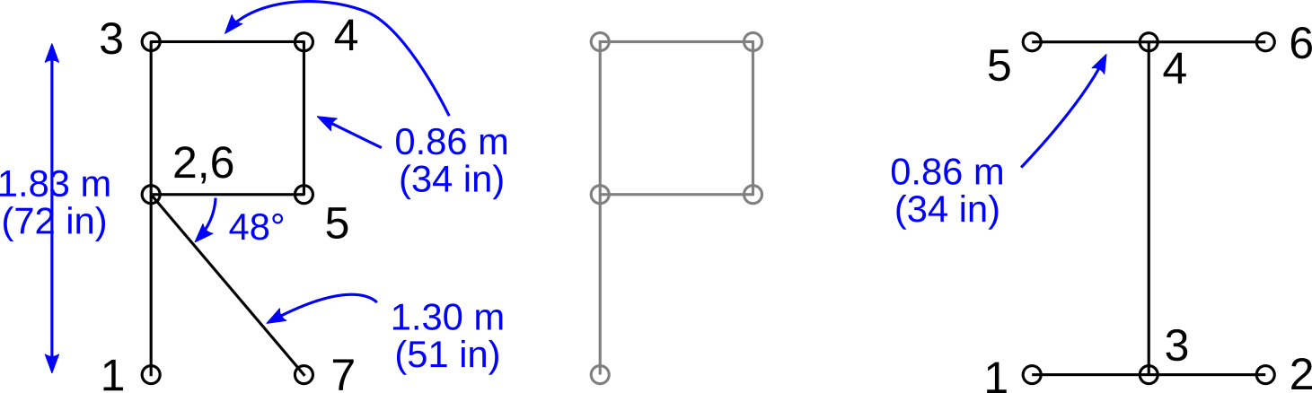
Paths to follow.
For both paths, the car is to start at location (1) and travel to the numbered locations in order until it reaches the end of the path, at which point it should stop. The car should drive straight forward between the numbered locations, using the motor encoders to determine how far to drive and when to stop. When at a numbered location, the car must turn on the spot in order to prepare for driving straight towards the next waypoint. The car is expected to be able to achieve this functionality at any speed, though the accuracy of the driving will likely be better at lower speeds (lower PWM duty cycles).
The direction and speed of the motors must be controllable to achieve these requirements. As discussed in Timer Compare: Motor PWM, the motors on the car are connected through an H-bridge chip (DRV8838) such that no hardware needs to be built for this application. The connections on the RSLK are as shown in the figure below.

Wiring of motors on RSLK
This lab requires that a PWM with a duty cycle between 25 % and 50 % be applied to the DRV8838 drivers, while the direction lines are manipulated to cause the car to either drive straight (both directions lines high) or turning without moving (one direction line high, one direction line low). The drive PWM frequency should be 40 kHz.
As the desired speed of the wheels will likely not be consistent between both wheels when given the same PWM duty cycle, it is necessary to measure the rotational speed of each and adjusting one, or both, PWM outputs such that the resultant speeds are equivalent; otherwise, the car will tend to turn left or right when it should ideally be traveling straight. To this end, the motor encoders will be used to accurately measure the wheel speeds.
Without the encoder measurements, the control of the wheel speed would be considered a type of Open-Loop Control; where the output is calculated blindly (without knowledge of the actual speed), usually based on system models. For example, a crude system model may assume that speed is linear with PWM duty cycle: 50 % speed would correspond to 50 % duty cycle; however, the model doesn’t take into account friction or drive inclination, etc. Adding the encoder measurements to inform the PWM output is considered a type of Closed-Loop Control, where the encoders are part of a feedback path for the control loop:
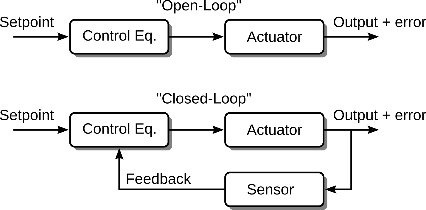
Open-Loop vs. Closed-Loop Control
As shown, the feedback in a closed-loop control is a measurement of the output which augments the drive signal; used to account for deviations (errors) from the desired setpoint or to adjust other response features. A common implementation of control in this manner is Proportional, Derivative, and Integral Control, or PID, which is a future topic in this course. For the application of this lab, a rudimentary control scheme will be implemented that will simply increase or decrease the drive signal to the motors incrementally until the desired speed is reached.
In addition to using the encoders to ensure the motors are operating at the same speed, they will also be used to measure the travel distance to determine if the car has either drove the required distance or turned the appropriate amount.
Part A: (Class 1) Driving Straight
The PWM and encoder programs produced for the previous two activities: Timer Compare: Motor PWM and Timer Capture: Motor Encoders, should be combined such that both the PWM generation and encoder measurements happen within the same program. Once combined, the program should be modified to ensure that the RSLK can drive in a straight line, implemented as described below.
Important
Activities 10 and 11 should have been completed using different timers if following the instructions correctly. When combining the activities; ensure that the timer modules used to generate PWM and measure the encoders do not use the same timer module.
In order to cause the car to drive straight, the wheels must be forced to drive at the same speed. To this effect, a simplistic control scheme is proposed. A rigorous calculation of the wheel speed may be done to provide the speed in a specific unit (e.g., rpm); however, as long as it may be assumed that the encoder/motor/gear-train/wheel assemblies are physically identical, then the only quantity required to characterize the wheel speed is the timer count difference between each encoder edge.
Assuming a desired wheel speed of xxx timer counts (timer counts between encoder edges), a logical comparison may be made on whether the wheel is rotating too slow or too fast. If it has been determined that the wheel is spinning too slow, then the drive PWM should be increased by a single PWM timer count; likewise, if the wheel is spinning too fast, the drive PWM should be decreased by a single PWM timer count.
To reduce the effect of normal variations in the measurements on the control scheme, a set of six wheel speed measurements should be averaged together for each PWM update. Sample pseudocode for this control scheme is provided below.
Variables required:
    A variable to track timer counts between encoder edges <-- Done in Activity 11
    A variable to store summation of wheel speed (timer counts) measurements <-- For averaging
    A variable to track number of measurements in the summation variable     <-- For averaging
    A variable to store the current PWM (or can be read from CCR)

<in CCR ISR>
    ...
    Calculate the counts between edges <--Done in Activity 11
    Sum result with previous results
    Add 1 to variable tracking number of results in sum
    if sum tracking variable == 6
        If sum variable / 6 > setpoint
            Subtract 1 (or Add 1) to PWM value
        If sum variable / 6 < setpoint
            Add 1 (or Subtract 1) to PWM value
        Apply PWM value
        reset sum tracking variable
        reset sum variable
Some notes on this implementation:
This code should be added within the timer interrupt for when a CCRn capture event occurs.
This process will need to be done twice: once for each motor. This implies that two versions of each variable must be created.
Subtracting/Adding to the PWM value depends on the TIMGx_Cn mode of the PWM: type 1 or type 2 as described in Timer Compare: Motor PWM. You will need to determine which is correct considering the mode (or test!).
The “setpoint” value in the pseudocode is a number of encoder timer counts to compare to (Not PWM timer counts!). It has been found that a value of 80000 corresponds roughly to a 25 % duty cycle and 40000 to 50 %.
When the path driving state starts, the wheel PWMs should be set to the ideal desired duty cycle and then allowed to be adjusted via the routine above. That is, the initial value for the PWM duty cycle should be the ideal value.
For your initial implementation of this control, you must implement the algorithm for only one wheel control first with the other wheel off and disabled. Debugging both wheels at the same time is very difficult. Verification of single wheel operation may be done by printing out the desired and actual speeds (in unit: timer counts) and ensuring that the actual speed converges to the desired speed. After the first wheel control is completely implemented, copy the code and make the necessary changes to control the other wheel; also independently verifying.
Warning
Be aware that the CCRn instances used for a single motor and encoder will not be the same number! For instance, if the PWM is applied on CCR0, then the encoder will be acting on CCR1. This is due to how the GPIO pins are routed on the RSLK.
Note
As noted, the suggested “setpoint” values given above are desired wheel speeds, but are given in terms of timer counts. The effective speed can be calculated from the velocity equation given in Timer Capture: Motor Encoders, where the setpoints of 80000 and 40000 timer counts correspond to physical speeds of ~250 mm/s and ~500 mm/s, respectively.
The wheel speed should be averaged over 6 measurements due to the construction of the encoder: the spinning magnet is not a single N-S pole pair (as shown in Timer Capture: Motor Encoders but instead has a set of 6 N-S pairs); which are not perfectly arranged around the disk. A 6 measurement average removes any inconsistances in the poling.
Similarly, the gear train between the motor (and magnetic disk) is a 60:1 ratio. This ratio is multiplied by 6:1 due to the 6 N-S pairs, resulting in the 360:1 encoder-to-wheel ratio.
Checkoff
Demonstrate that the car may drive in a straight line. The car is allowed and may be expected to turn slightly when the program starts due to initial errors between the wheel speeds. The car will drive straight once the routine above has been evaluated many times (< 1 s).
Part B: (Class 2) Follow the Path…
The driving control must be added to the speed control developed in Part A. A possible state diagram for the system is provided in the figure below.
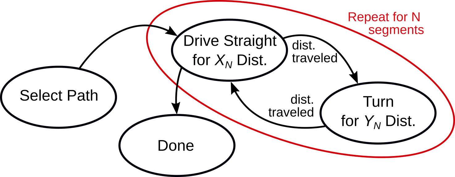
Lab 3 state diagram
The first state in the program is to simply wait until either the “R” or “I” path is selected. This is done with two bumpers: one to select each path. When one of these bumpers is pressed, the program should wait for the button to be released and then will attempt to navigate the path.
Hint
As proposed in the state diagram, the “Drive Straight” and “Turn” states are repeated N times for each segment of the path; where each state needs to run for a predetermined distance (XN and YN). This lends itself very well to storing the values for XN and YN within one or two arrays for each path. The path selection can then be done by passing the desired array(s) to a Drive() function:
void Drive(uint16_t * distances);

uint16_t pathA[] = {...};
uint16_t pathB[] = {...};

void main(){
    ...
    Drive(pathB);
    ...
}

void Drive(uint16_t * distances){
    // Loop through elements of array "distances"
}
Of course, this example code only considers using one array per path. This approach could easily be extended to using two arrays by adding a second argument to the function Drive().
It is not required that you implement your code this way, this is just a suggestion.
Measuring Turn Angle
The drive distance calculation for driving straight forward is simple and should be understood from Activity 11; however, calculation of the car turn angle can be a complicated kinematics problem. To simplify this problem, we will make the assumption that the car will turn perfectly about its center. The geometry involved in this calculation is provided in the figure below.
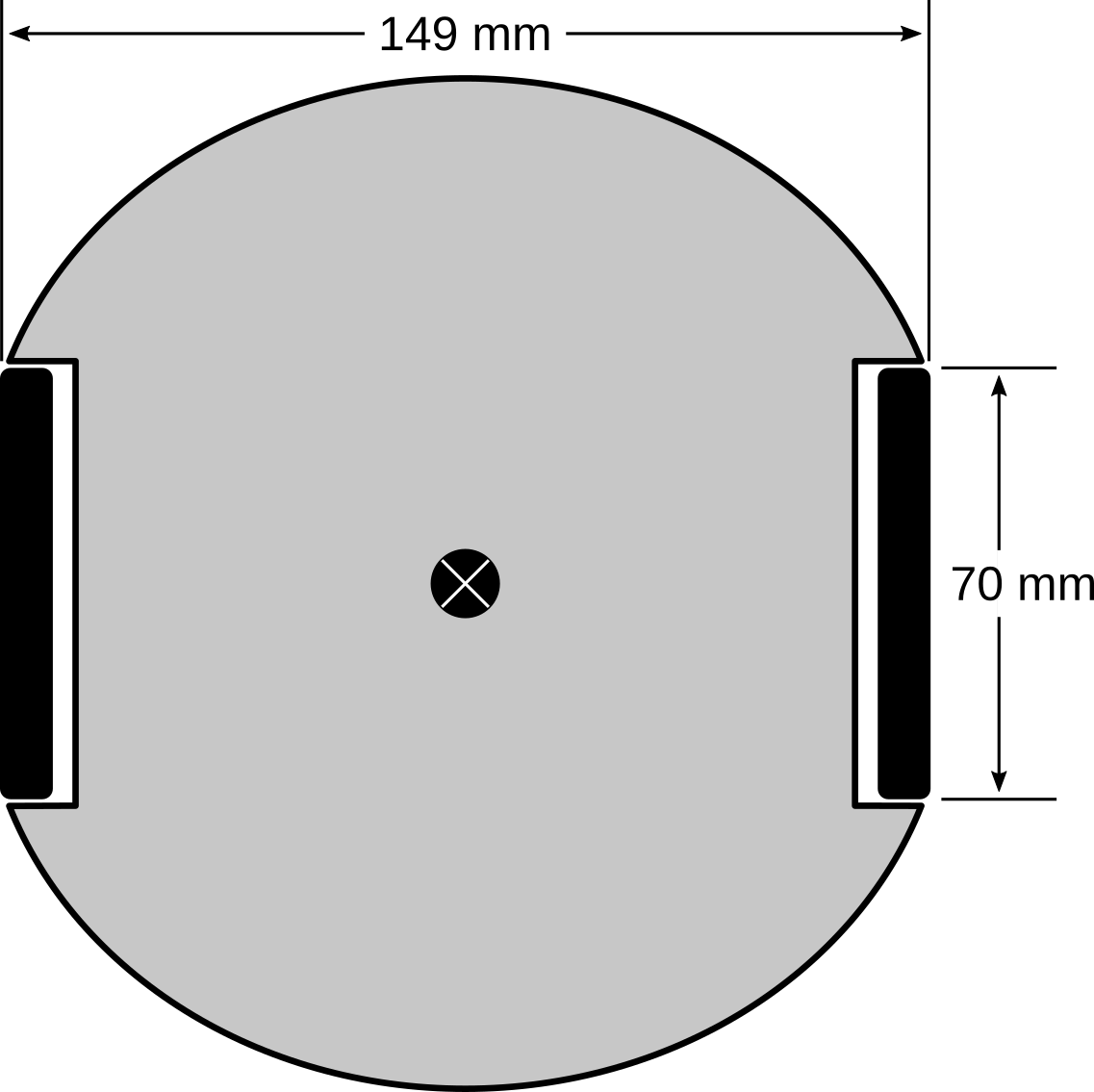
RSLK geometry and dimensions
If the RSLK is rotating about the center point marked, then the center of the wheels must travel in a circle. Assuming no slip (on average), then the distanced measured by the encoder is a measurement of the arc length of the rotation, \(s\). This reduces the calculation down to the calculation of the angle, \(\theta\), from the encoder measured arc length, \(s\), and the distance from the car center to the wheel, \(r\):
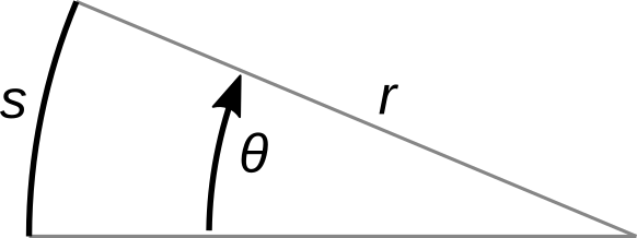
Arc length geometry
Hint
You may notice large errors in turning when using higher wheel speeds due to transients of the motors turning on and off or switching directions. To produce more accurate turns, you may use a lower PWM duty cycle than used when driving straight. If following this route, the speed control loop should be disabled for turns, with the corrected pulsewidths from previous instance of driving straight re-applied after turning is complete.
It is also possible to avoid the arc length math above by emperically determining the correlation between encoder events and rotation by allowing the car to turn many rotations while tracking the total encoder counts; then calculating the effective degrees rotate per encoder count via:
Checkoff
Demonstrate the RSLK is able to follow the “R” and “I” paths, selectable via a button press. The RSLK is not expected to perfectly follow the paths, but should reasonably resemble the “R” and “I” on the floor as marked. General guidance: if the RSLK finishes the letter within approximately 30 cm or so of the endpoint it is usually acceptable.
Warning
Be aware that the floor is not perfectly flat (especially on the long edge of the “R”), which will cause the RSLK to veer off course even with a correct control implementation; this effect does not need to be accounted for, other than possibly manually nudging to correct.
Submit the code used for the checkoff to Gradescope.